Gradient Descent and Backpropagation: How Neural Networks Learn
The loss measures how wrong a model is. Backpropagation works out how much each weight contributed to that error. Gradient descent moves each weight a small step to reduce it.

Training a neural network is a loop. A forward pass runs an input through the network to produce a prediction. A loss function turns the gap between prediction and target into one number. Backpropagation then works out, for every weight, how a small change would move that number. Gradient descent uses those answers to nudge each weight a small step in the direction that lowers the loss.
The two terms are often used interchangeably, but they do different jobs. Backpropagation computes gradients. Gradient descent uses them to update the weights. Most optimisers used for deep learning, including Adam, are variations on the second step, fed by the first.
The loss: one number for being wrong
Training needs a target. For a model that predicts a number, a common loss is the squared error: the square of the difference between prediction and target. Averaged over a dataset, it becomes one number that falls as predictions improve. Classification networks usually use cross-entropy instead, which penalises confident wrong answers heavily. Whatever the loss, its value is the quantity the optimiser tries to reduce.
Gradient descent: step downhill
A gradient is the slope of the loss with respect to one weight: how much the loss changes if that weight increases by a tiny amount. A network has one gradient per weight, collected into a vector. The gradient points in the direction in which the loss rises fastest, so the update subtracts it:
w_new = w_old - learning_rate * gradientStanford's CS231n course notes describe the idea as a blindfolded walker on a hill. You can feel which way is steepest, but you still have to choose how far to step. The step size, called the learning rate, is one of the most important hyperparameters in training a neural network (CS231n optimisation notes). A large step can make more progress, but it is riskier. For a large enough step the walker overshoots, and the loss gets worse instead of better.
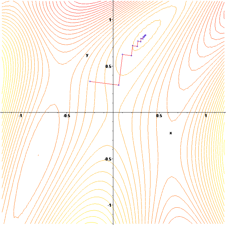

The playground's Gradient Descent tool plays this out on a surface you can click. Its learning-rate slider runs from 0.01 to 0.3 and starts at 0.05, so you can see the difference between a cautious step and an overshoot.
Backpropagation: the chain rule, run backwards
A neural network is a long chain of simple operations: multiply by weights, add, apply a nonlinearity, repeat, and finally compare the output with the target. The chain rule of calculus says that the derivative of a composed function is the product of the derivatives of its parts. Backpropagation applies that rule systematically to the whole chain.
The forward pass stores every intermediate value. The backward pass starts at the loss and walks back through the layers, multiplying local derivatives and accumulating the result into the gradient of each weight. Each intermediate result is computed once and reused, which is what makes the procedure efficient.
A 1986 Nature paper by Rumelhart, Hinton and Williams popularised the method. Its abstract describes back-propagation as a learning procedure that repeatedly adjusts the weights of the connections so as to minimise a measure of the difference between the actual and desired output vectors. As a result, hidden units that are neither inputs nor outputs come to represent important features of the task (Rumelhart et al., 1986).
Why not estimate each gradient by nudging each weight and re-running the network? The CS231n notes point out that evaluating the numerical gradient has a cost linear in the number of parameters, which is impractical for networks with millions of weights. The analytic gradient from the chain rule, which is backpropagation, avoids that cost.
A worked example in three steps
Take one weight w, one input x = 2 and one target t = 3. The model predicts y = w × x, and the loss is L = (y − t)². Backpropagation on this tiny graph is the chain rule: dL/dw = (dL/dy) × (dy/dw) = 2(y − t) × x. Start with w = 0.5 and use a learning rate of 0.1.
| Step | w | y = w × x | L = (y − t)² | dL/dw = 2(y − t) × x | New w = w − 0.1 × dL/dw |
|---|---|---|---|---|---|
| 1 | 0.50 | 1.00 | 4.0000 | −8.00 | 1.30 |
| 2 | 1.30 | 2.60 | 0.1600 | −1.60 | 1.46 |
| 3 | 1.46 | 2.92 | 0.0064 | −0.32 | 1.492 |
Each step cuts the loss by a factor of 25 here: 4, then 0.16, then 0.0064. The distance between w and the ideal value 1.5 shrinks by a factor of 0.2 at every step.
Now try a learning rate of 0.5. The same gradient of −8 moves w to 4.5, the prediction jumps to 9 and the loss rises to 36. For this loss, each update multiplies the distance to 1.5 by 1 − 2 × η × x², which is 0.2 at η = 0.1 but −3 at η = 0.5. The weight therefore oscillates further away on each step. This is the overshoot that the CS231n notes warn about.
Why one backward pass is enough
The efficiency of backpropagation is the reason it matters. Estimating gradients numerically means nudging each parameter and re-running the network, so the cost grows with every weight. For a network with a million weights, one update would need about a million extra evaluations. Backpropagation gets every partial derivative from one forward pass and one backward pass. That difference is what makes training networks with millions of weights practical.
Mini-batches: noisy steps are cheap
Computing the gradient over the whole training set before every step is expensive. Stochastic gradient descent estimates it from a single example, and mini-batch gradient descent from a small random batch. Each estimate is noisy, but many cheap steps are often more useful than a few exact ones. Ruder's overview of gradient descent algorithms covers the batch, stochastic and mini-batch variants and the trade-offs between them (Ruder, 2016).
Where Adam and normalisation fit
Plain gradient descent uses one learning rate for every weight. Adam keeps running averages of each weight's gradient and of its square, and uses them to scale that weight's step. Its authors describe it as an algorithm based on adaptive estimates of lower-order moments (Kingma and Ba, 2014). It is still gradient descent with a smarter step. The Adam report on this site walks through the update rule.
The chain rule multiplies one local factor per layer. If those factors are consistently below one, the gradient reaching the early layers shrinks. If they are consistently above one, it grows. Architecture and initialisation choices exist partly to manage this. Residual connections in ResNet give the gradient a short path through very deep stacks. He initialisation sets the scale of the starting weights for ReLU networks so that signal variance stays stable. Normalisation layers such as Batch Normalization and Layer Normalization rescale activations inside the network, which changes how safely the optimiser can take large steps.
Try it in the playground
Two playground tools map onto this post. The Gradient Descent tool moves a ball across a surface using the learning rate you set. The Backpropagation tool animates a small two-layer network, with forward signals in steel blue and backward error signals as dashed vermilion lines. Use the worked example to predict what a large learning rate does, then set a high rate on the Gradient Descent tool and watch the ball overshoot.
For the wider context, the training topic hub and the architectures topic hub list the reports that use these ideas. The about page explains how this site checks the claims in its reports.
References
- Rumelhart, D. E., Hinton, G. E. and Williams, R. J. (1986). Learning representations by back-propagating errors. Nature 323, 533–536: https://www.nature.com/articles/323533a0.
- Ruder, S. (2016). An overview of gradient descent optimization algorithms. arXiv:1609.04747: https://arxiv.org/abs/1609.04747.
- Kingma, D. P. and Ba, J. (2014). Adam: A Method for Stochastic Optimization. arXiv:1412.6980: https://arxiv.org/abs/1412.6980.
- Stanford CS231n. Optimization, part 1 (course notes, backpropagation and gradient descent): https://cs231n.github.io/optimization-1/.
- Goodfellow, I., Bengio, Y. and Courville, A. (2016). Deep Learning. MIT Press. Chapter 8, optimisation for training deep models: https://www.deeplearningbook.org/contents/optimization.html.
This guide is an explainer, not peer-reviewed research. Check the linked primary sources before relying on any specific claim.
Frequently asked questions
What is the difference between gradient descent and backpropagation?
Backpropagation computes the gradient of the loss with respect to every weight, using the chain rule. Gradient descent uses those gradients to update the weights. Standard neural network training needs both.
What is a gradient, in plain terms?
It is the slope of the loss with respect to one weight: how much the loss changes if that weight is nudged up a little. The gradient points uphill, so the update moves the other way.
Why does the learning rate matter so much?
It sets how far each update moves. Too large and the loss overshoots, as the worked example shows, and can get worse. Too small and training needs a great many steps (CS231n optimisation notes).
Does gradient descent find the best possible weights?
Not in general. For convex problems, any local minimum is a global minimum. Neural network losses are nonconvex, where local minima can cost more than the global minimum, and saddle points are common in high-dimensional problems (Goodfellow et al., 2016, chapter 8). In practice, trained networks often work well anyway.
How does Adam differ from plain gradient descent?
Adam keeps running averages of each weight's gradient and squared gradient, and uses them to scale that weight's step. It is still a gradient-based update (Kingma and Ba, 2014). The Adam report on this site covers the details.